

In any process, the measurement of electricity is essential for monitoring, analyzing and controlling the system. To perform these types of measurements, current sensors must be used. Physical quantities cannot be managed unless they can be measured. Let’s dive into the behavior of the current sensor.
What is Current Sensor?
A current sensor is a device that converts a current signal into another signal that can be analyzed. The signal to be measured is called “primary current” and the output signal is called “secondary current or voltage”. The last signal is for electronic boards, ADCs, and other analog instruments. Since different measurement techniques exist, and the primary current can vary by waveform, pulse type, isolation, and current strength, the market offers a variety of current sensors. As shown in Figure 1, the most common current sensors fall into two categories:
According to the working principle of “shunt”, the first type applies Ohm’s law ( V = R × I ).
The second class uses Ampere’s law (I = ∮ H × ds) and uses a magnetic field to measure current.
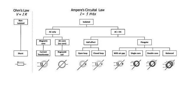
Figure 1: Different current measurement methods
Ohm’s law applies to shunt measurements with the formula V = R × I. In practice, a shunt is a robust resistor with a known ohmic value. When current flows through the shunt, the resulting voltage is proportional to that current. Using this principle, for currents that are not too high, we can get AC and DC currents accurately. On the other hand, when the current rises and exceeds 100 A, too much heat is generated and the measurement system can become ineffective and critical.
Hall-effect current sensors can be used to overcome these limitations. Powering a Hall probe applies a magnetic field perpendicular to the surface and produces a voltage proportional to the strength of the magnetic field. The amount of current flowing through the conductor can then be calculated using Ampere’s law. Hall current sensors use a magnetic core to concentrate the magnetic field in the air gap where the probe is located. The output voltage is proportional to the magnetic field, which in turn is proportional to the primary current. The performance of the current sensor depends on the performance of the open loop Hall probe. In order to improve the linearity and reduce the drift of temperature offset, the closed-circuit principle is implemented, and another current sensor is represented by a magnetoresistor, where the value of the resistor changes proportionally to the magnetic field. These current sensors are generally more accurate than the Hall effect, but have sensitivity limitations due to the air gap. However, the equipment must ensure efficient and accurate measurements with very high detection quality, extremely flat frequency response and excellent DC stability. All of these characteristics can be found in Danisense’s current sensors, the company offering customized solutions to meet the exact needs of customers.
Current Measure Method
Current measurements can be performed using the LT6106 integrated circuit, a multifunctional amplifier for current sensing (see the application diagram in Figure 2). Its features are highly regarded:
Maximum Voltage Offset: 250 µV
Maximum Input Bias Current: 40 nA
Only two resistors are needed to set the gain of the device
Accuracy: 1%
Maximum output current: 1 mA
PSRR: 106 dB
Its main applications are automotive and industrial, battery monitoring, energy management, engine control, lamp monitoring, and overcurrent and fault detection. The device measures current by detecting the voltage across an external resistor (shunt resistor). Internal circuitry converts this voltage to output current. The very low supply current of the LT6106 also makes it suitable for battery applications.
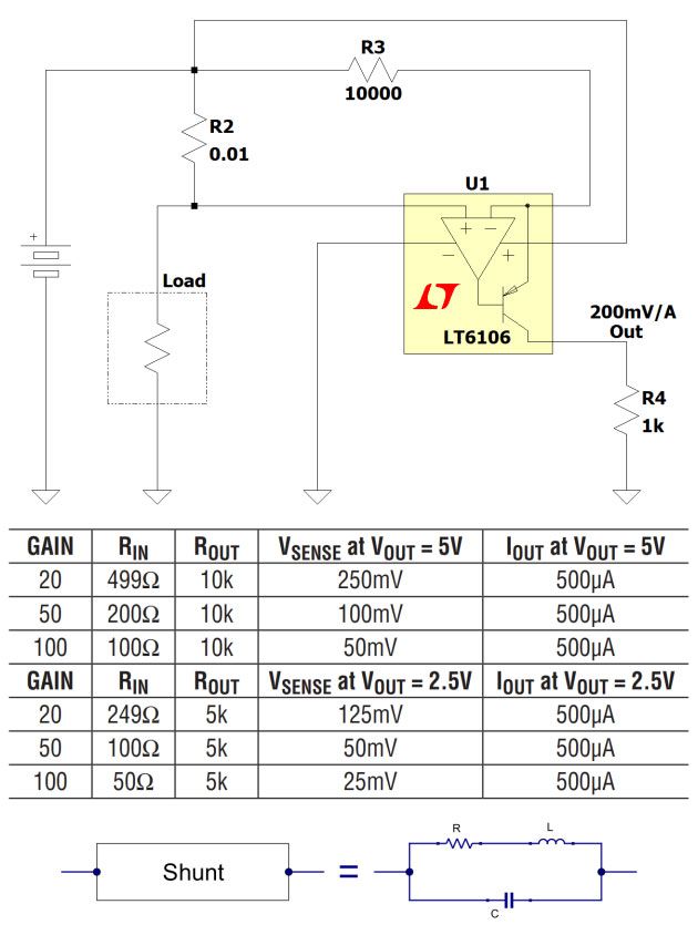
Figure 2: Example of a load current table using the LT6106 device
Once you understand how it works, you can easily configure the design to meet all your needs using Ohm’s law and power equations. In the example wiring diagram configuration, the power supply is 30 V and powers a 19-Ω load at approximately 1.57 A. The 0.01-Ω shunt resistor does not affect the operation of the system, which dissipates approximately 25 mW. Configure the configuration resistor to make the gain of the amplifier unity. In this case, the output voltage (in absolute value) is equal to the current flowing through the load. The overall efficiency is very high, definitely more than 99.8%. Obviously, this solution cannot be used for very high currents.
Current Sensor vs Shunt
Using a current sensor instead of a shunt has great advantages. A shunt, in fact, is not an ideal component, but as you can see from the previous wiring diagram, it has an inductive element (in series) and a capacitive element (in parallel). So current measurements need to be made not only in DC but also in AC so there needs to be a more efficient method to make better estimates in different frequency and current ranges for higher results accuracy.
Current sensors have the advantage of electrically isolating the primary circuit from the secondary circuit. This eliminates interference from common-mode voltage ripple and greatly reduces noise on the primary current. Compared to shunts, current sensors have higher output signals and lower noise. The much lower insertion impedance reduces power consumption and undoubtedly improves the short- and long-term stability of the system.
A simple example illustrates the idea: a shunt resistor to provide 50 mV at 1,500 A dissipates 75 W. In fact, it has an impedance of 0.000033 Ω. To achieve high measurement stability and repeatability, the shunt requires a very low temperature coefficient. Sensitivity in Volts/Amps will vary if the system is used at low or high current. For example, the effective insertion impedance of the DL2000UB-10V current sensor is less than 0.5 µΩ, and the effective power dissipation in the primary circuit is less than 1 W at 1,500 A, which is 100 times less than the previous shunt. Even with very low primary current, the signal-to-noise ratio is very high. The table in Figure 3 shows an excerpt from the Danisense current sensors of the DS, DM, DL and DQ series. These sensors are ultra-stable and highly accurate, and based on closed-loop operation, they provide excellent linearity and stability over time.
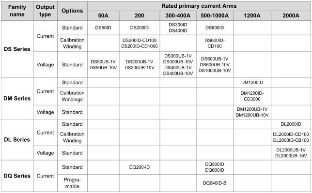
Figure 3: DS, DM, DL, and DQ Series Transducer Models
Broadly speaking, some models of transducer combinations can be divided into the following categories:
Sensors from 0 A to 600 A
DP50IP-B (72A)
DC200IF (300A)
DS400ID (600 A)
DS50UB-1V (150 A)
Sensors from 600 A to 3,000 A
DM1200ID (1,800 A)
DL2000ID (3,000 A)
DL2000ID-CB100 (3,000 A)
DL2000UB-10V (2,200 A)
Sensors greater than 3,000 A
DR5000IM (8,000 A)
DR10000IM (11,000 A)
DR5000UX-10 V/7,500 A (8,000 A)
Some of them provide current output while others provide voltage. One of the many interesting models is the DM1200UB-1V (Figure 4), an ultra-stable and high-accuracy sensor for measuring non-intrusive and isolated DC and AC currents up to 1,800 A. Its opening has a diameter of 45 mm, a width that allows large insulated cables and the possibility of measuring leakage currents with high precision. With 15 ppm linearity and 10 ppm offset, its closed-loop technology enables very accurate measurements. The body is made entirely of aluminum for improved EMI shielding and wide operating temperature. Its applications range from power measurement and analysis to the construction of stable power supplies, from particle accelerators to precision drives, from battery test and evaluation systems to power system calibration. Here are some electrical characteristics of the device:
Rated primary AC current: max. 1,200 weapons
Nominal Primary DC Current: Max. 1,200 A
Measurement range: from –1,800 A to 1,800 A
Nominal Voltage Output: –1 V to 1 V
Primary/secondary ratio: 0.8333 V/kA
Linearity Error: From –15 ppm to 15 ppm
Bandwidth (3 dB): 400 kHz
Amplitude Error (10 Hz to 3 kHz): 0.01
Amplitude Error (3 kHz to 50 kHz): 1
Amplitude Error (50 kHz to 300 kHz): 20
Supply Voltage: ±14.25 V to ±15.75 V
Positive current consumption: 140 mA
Negative current consumption: 130 mA
Operating Temperature Range: –40˚C to 65˚C
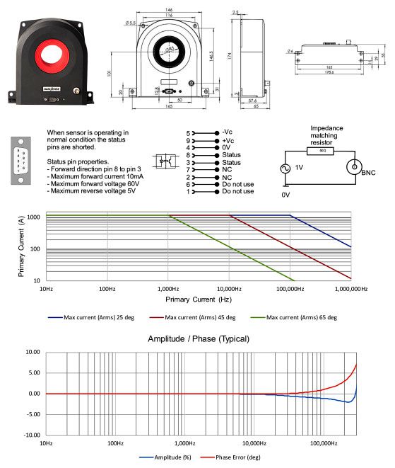
Figure 4: DM1200UB-1V sensor
Conclusion
Today, all industrial systems have current sensors, and in some cases they are irreplaceable. Their main advantage is that they can be used and easily interpreted by industrial control systems and are completely isolated from circuits and loads. In fact, it is not always convenient to connect the measurement system directly to the relevant circuit. Their footprint is non-invasive, and they typically have a square or rectangular shape that may resemble a small speaker. However, their function is very important. The engineering behind the transducer operation is quite complex, but its operation and analysis of the output data is extremely simple, which is the most important aspect.
Author: Aidan Taylor
Website: https://reversepcb.com/